1: Shannon’s Demon, Made Exact

How to make an exponential amount of money from a portfolio of lemons without shorting anything

Introduction

If intuition is any guide, it shouldn’t be possible for a long-only portfolio to be profitable when each of its component assets is a lemon, unless, of course, one is clairvoyant and can predict those fleeting moments when random chance will favor each asset. Yet, as I’ll demonstrate in this post, not only is it possible to do this without any clairvoyance whatsoever, but also an investor can (almost surely) guarantee an exponential amount of money in the long run from an appropriately constructed portfolio of such lemons, at least under certain conditions that this post makes exact. It turns out that information theory provides a lovely explanation for why this is possible. The culmination of this post is a simple, closed-form formula for the excess expected growth rate of a portfolio over the risk-free rate, for a two-state, two-asset complete market. This formula is expressed as the difference between two Kullback-Leibler divergences.

Figure 1: Vincent van Gogh, Still Life with Lemons on a Plate, 1887. Van Gogh Museum.

Maxwell’s demon and Shannon’s demon

Named after the legendary physicist James Clerk Maxwell, Maxwell’s demon is a thought experiment in physics in which a hypothetical demon controls a microscopic, frictionless door separating two chambers of gas. The demon selectively sorts fast and slow molecules in the gas to pass through the door so that the fast molecules go to one chamber and the slow molecules go to the other, thereby creating a temperature difference without expending any of the system’s energy. This procedure would lead to an increase in the free energy of the system, which could then be used to do useful work, seemingly violating the second law of thermodynamics. Put differently, the demon extracts useful work from heat, which is the random energy of the molecules, all at no apparent thermodynamic cost to the system. This is magic for a physicist, and like magic, it is impossible. The modern resolution of this paradox is that there is in fact a cost to the system, as the demon with its finite memory must eventually erase its records, and erasing information dissipates at least \(k_B T \ln 2\) of heat per erased bit, creating entropy in the process (Landauer 1961; Bennett 1982).

In a nod to Maxwell’s demon, Shannon’s demon, which is named after the founder of information theory, Claude Shannon, is a somewhat analogous thought experiment in investing in which the random up-and-down noise of asset prices (loosely analogous to heat in physics) can seemingly “magically” create wealth by rebalancing one’s portfolio in just the right way so as to maximize the long-run growth rate (Cover 1998). It is as if Shannon’s demon is able to sort profitable outcomes from unprofitable ones. Unlike Maxwell’s demon, however, Shannon’s demon exists in the sense that it is a real, mathematically rigorous strategy that does not violate any laws of physics or finance. The connection to thermodynamics is purely one of loose analogy; the actual concepts are information-theoretic.

Alexandre Cabanel, Fallen Angel, 1847. Musée Fabre.

The setup

In order to most clearly illustrate the concepts at play, I have necessarily chosen a very simple (and therefore unrealistic) example, in which there are only two assets to invest in: a risk-free asset with a negative interest rate and a risky asset modeled by a coin flip. Nonetheless, the results and machinery I develop here generalize to more realistic settings, though of course there are additional nuances and complications that arise in those cases, such as estimating return probabilities, accounting for transaction costs, and so on. In this post, however, I will ignore such complications in order to focus on the core ideas.

We will think of the risk-free asset as reminiscent of a Swiss bank account: the account is so safe and so desirable that it pays a negative interest rate; hence, its associated gross return satisfies \(r < 1.\) On the other hand, the risky asset, which I’ll model as a coin flip, will be highly volatile in its outcome, where heads comes with a very handsome (gross) return of \(\gamma_h\) with probability \(0 < p_h < 1\) and tails with a very steep loss \(\gamma_t < r < \gamma_h\) (with probability \(1 - p_h\)). In addition, I’ll set \(\gamma_t = \alpha / \gamma_h\), for some \(\alpha > 0\), i.e. \(\alpha = \gamma_h \gamma_t\) is the gross return of one heads-and-tails round trip. Finally, I let \(f\) denote the fraction of our money that we allocate to the risky asset (hence, \(1 - f\) is the fraction that we allocate to the risk-free asset). After every period, we rebalance our portfolio to maintain these fractions. If we disallow shorting the risky asset, then we limit ourselves to \(f \geq 0\), and if we disallow leverage (shorting the risk-free asset), we require \(f \leq 1\). Our goal is to choose \(f\) intelligently so that we make as much money as possible in the long run (or lose the least possible).¹ I’ll let \(S_0\) denote the initial wealth.

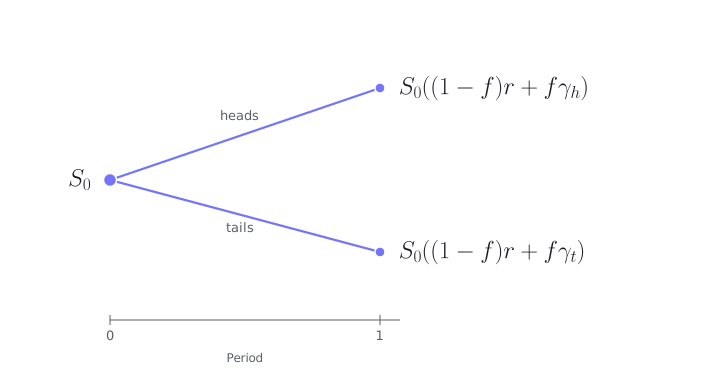
In what follows, let \(w^T = (1 - f, f)\) denote the allocation vector and \(X^T = (r, \gamma)\) the random gross returns vector, where \(\gamma\) takes the value \(\gamma_h\) with probability \(p_h\) and \(\gamma_t\) with probability \(1 - p_h\). Note that \(w^T = (1,0)\) corresponds to a portfolio consisting solely of the risk-free asset, and \(w^T = (0,1)\) corresponds to a portfolio consisting solely of the risky asset. The portfolio gross return for a particular period is then given by \[Y(w) = w^T X = (1 - f)r + f\gamma,\] so the wealth after \(n\) periods is \[S_n(w) = S_0\prod_{i=1}^n Y_i(w),\] where \(Y_i(w)\) is the portfolio gross return in period \(i\). This multiplicative branching of wealth, starting from the initial wealth \(S_0\), is sketched in Figure 2.

Figure 2: The first period of the wealth tree. Starting from \(S_0\), a heads scales wealth by the portfolio gross return \((1-f)r + f\gamma_h\) and a tails by \((1-f)r + f\gamma_t\). The tree branches this way at every period, compounding multiplicatively.

For the specific example below, I’ll set:

1. \(r = 0.97\): a negative interest rate of 3% per period.
2. \(\gamma_h = 2\): a 100% net gain on heads.
3. \(p_h = 0.5\): it’s a fair coin.
4. \(\alpha = 0.8\): this implies \(\gamma_t = 0.4\), i.e. a 60% net loss on tails.
5. \(S_0 = 1\): initial wealth is normalized to 1.

from coin_flip_with_riskless_asset_model import CoinFlipWithRisklessAssetModel
coin_flip_model = CoinFlipWithRisklessAssetModel(r=0.97, gamma_heads=2.0, p=0.5, alpha=0.80)

The risky asset is a lemon

Obviously the risk-free asset is a lemon, as it bleeds 3% each period. (By “lemon” I simply mean an asset that will almost surely grind its way to a 100% loss over time.) While it is less obvious, the risky asset is also a lemon, which can be seen using Monte Carlo simulations.

import numpy as np
from finlib.ensemble_of_returns_paths import EnsembleOfReturnsPaths # finlib: https://github.com/jordanmckittrick/finlib
from finlib.simulating_performance import crp_performance # finlib: https://github.com/jordanmckittrick/finlib

seed = 12345
rng = np.random.default_rng(seed)
num_paths = 10_000
num_periods = 500

weights_for_risky_asset = np.array([0.0, 1.0]) # 0% in risk-free, 100% in risky
gross_returns_tensor = coin_flip_model.generate_random_gross_returns(rng, num_periods=num_periods, num_paths=num_paths)
perf_risky_matrix = crp_performance(weights_for_risky_asset, gross_returns_tensor)
ensemble_risky = EnsembleOfReturnsPaths.from_gross(perf_risky_matrix)

growth_rate_summary_df_risky = ensemble_risky.summarize_across_paths(ensemble_risky.running_growth_rate, threshold=0.0) 
wealth_summary_df_risky = ensemble_risky.summarize_across_paths(ensemble_risky.running_wealth_ratio, threshold=1.0) 

Figure 3 summarizes 10,000 simulated wealth paths over 500 periods (coin flips) for the risky asset. The shaded region indicates the middle 95% of these wealth paths.

Figure 3: Simulated wealth paths for a portfolio held entirely in the risky asset. Top: wealth as a multiple of starting wealth, drawn on a logarithmic scale, with the empirical median, the empirical mean, and the middle 95% of paths (300 paths shown). Not shown: the expected value path. The empirical mean underestimates the true expected value at any feasible number of paths, as the latter is carried by extremely rare paths. Bottom: the fraction of paths still above break-even.

Clearly the typical path through log-wealth space is downward sloping in the long run (top panel of Figure 3). In addition, after only 100 coin flips, we see that fewer than 10% of the paths have made money, and after 250 flips, that fraction has fallen to just over 1%. After all 500 flips, it is essentially zero (bottom panel).

Indeed, the wealth path tends to zero with probability one. To see this, we begin with the observation that since the sequence of random variables is i.i.d., the strong law of large numbers implies that the empirical growth rate, \(W_n\), converges almost surely to the expected growth rate \(W(w)\) (which I’ll also simply call the “growth rate”): \[ \begin{align} W_n(w) &:= \frac{1}{n} \ln \left(\frac{S_n(w)}{S_0}\right) \\ &= \frac{1}{n} \sum_{i=1}^n \ln Y_i(w) \\ &\rightarrow \mathbb{E}\left[\ln Y(w)\right] \\ &=: W(w), \end{align} \] which defines \(W(w)\) in nats per period. For the risky asset, our weights vector is \(w^T = (0,1)\); hence, \[ \begin{align} W_n(w) &\rightarrow p_h \ln \gamma_h + (1 - p_h) \ln \gamma_t \\ &= \frac{1}{2} \big(\ln \gamma_h + \ln \gamma_t \big) \\ &= \frac{1}{2} \ln \alpha \\ &< 0, \end{align} \] since \(\alpha < 1\). Let \(x\) be any number satisfying \(\ln \sqrt{\alpha} < x < 0\). Then, by the definition of almost sure convergence, with probability one there exists some positive integer \(N\) such that for all \(n > N\), we have \(W_n(w) < x < 0\). This implies that for \(w^T = (0,1)\) we have \(S_n(w) = e^{n W_n(w)} < e^{n x} \rightarrow 0\) with probability one, which proves the claim that the risky asset is indeed a lemon.

Note that this result implies that, regardless of the starting allocation, any buy-and-hold strategy for these two assets will, with probability one, tend to a 100% loss in the long run, as the wealth of a portfolio adopting the buy-and-hold strategy is just a convex combination of the wealth of each asset in the portfolio: every buy-and-hold strategy is also a lemon. In order to avoid this fate, we will need to adopt a different strategy. In this post, I will consider the strategy of rebalancing our portfolio to some fixed value of \(f\) after every period, not allowing \(w\) to drift with the asset prices. The resulting portfolio is called a constant rebalanced portfolio (CRP). The question then becomes: what is the optimal value of \(f\)?

The expected wealth is a mirage

The expected value path for the risky asset, however, tells a very different story from the typical path. After 500 periods, the expected value path (not shown in Figure 3) for the risky asset sits around \(4 \cdot 10^{39}\), which is many orders of magnitude better than both the sampled median and the sampled mean, both of which are shown in the figure. This is because of the small number of rare paths with enough heads to make a killing. In fact, using the independence of the coin flips, we see that the expected wealth after \(n\) periods diverges to infinity exponentially fast: \[ \begin{align} \mathbb{E}[S_n] &= \mathbb{E}\left[S_0 \prod_{i=1}^n Y_i\right] \\ &= S_0 \prod_{i=1}^n \mathbb{E}[Y_i] \\ &= S_0 \prod_{i=1}^n \mathbb{E}[\gamma_i] \\ &= S_0 \mathbb{E}[\gamma]^n \\ &= S_0 \big(p_h \gamma_h + (1 - p_h) \gamma_t \big)^n \\ &= 1 \cdot 1.2^n \\ &\rightarrow \infty. \end{align} \]

Given that a wealth path tends to zero with probability one, the expected value path is a mirage, as the expected value is dominated by a small number of rare events, which are not representative of the typical outcome.

Figure 4: Thomas Moran, The Mirage, 1879. Stark Museum of Art.

Let’s now consider the probability that the path after \(n\) periods at least hasn’t lost any money, i.e. that \(S_n \geq S_0 = 1\). For this simple model, we can actually compute this probability exactly. Letting \(k\) denote the number of heads in \(n\) flips, we have \[ \begin{align} \mathbb{P}(S_n \geq 1) &= \mathbb{P}(W_n \geq 0) \\ &= \mathbb{P}\left(\frac{1}{n} \sum_{i=1}^n \ln \gamma_i \geq 0\right) \\ &= \mathbb{P}\left(\frac{k}{n} \ln \gamma_h + \frac{n-k}{n} \ln \gamma_t \geq 0\right) \\ &= \mathbb{P}\left(\frac{k}{n} \geq c \right) \\ &= \sum_{j=\lceil cn \rceil}^{n} \binom{n}{j} p_h^j (1 - p_h)^{n-j}, \\ \end{align} \]

where the critical fraction \(c = \frac{-\ln \gamma_t}{\ln \gamma_h - \ln \gamma_t} \approx{}\) 0.569 solves \(c \ln \gamma_h + (1 - c) \ln \gamma_t = 0\). For \(n = 500\), this yields \(\mathbb{P}(S_n \geq 1) \approx {}\) 0.001. On the other hand, we have \(\mathbb{E}[S_n] = 1.2^{500} \approx 4 \cdot 10^{39}\). So much for the expected value path being representative of the typical outcome.

To further underscore this point, we can compute an upper bound on this same tail probability by applying a Chernoff bound. The actual probability of heads is \(p_h = 0.5\), while the smallest empirical probability of heads that would yield a non-negative growth rate is \(\frac{\lceil c n \rceil}{n} \geq c\). Of all the empirical distributions of heads/tails that would achieve a non-negative growth rate, \(\left(\lceil c n \rceil / n, 1 - \lceil c n \rceil / n \right)\) is the “closest” to the actual distribution \((0.5, 0.5)\) in the sense of minimizing Kullback-Leibler divergence; however, it depends on \(n\). We can do away with the \(n\) dependence by observing that replacing \(\lceil c n \rceil / n\) with \(c\) would slightly decrease the KL divergence and thus very slightly weaken the Chernoff bound. Doing so, we find the resulting KL divergence, \(D_{\text{KL}}\), to be given by \[ \begin{align} D_{\text{KL}} &= c \ln \left(\frac{c}{p_h}\right) + \left(1 - c\right) \ln \left(\frac{1 - c}{1 - p_h}\right) \\ &\approx 0.00964. \end{align} \] The Chernoff bound then implies that \(\mathbb{P}(S_n \geq 1) \leq e^{-n D_{\text{KL}}}\), which decays exponentially in \(n\) (Cover and Thomas 2006, ch. 11). Figure 5 plots the exact tail probability against this bound.² In what follows, I will drop the “KL” subscript from \(D_{\text{KL}}\) and simply write \(D\) for the Kullback-Leibler divergence.

Figure 5: The probability of not having lost money after \(n\) coin flips, \(\mathbb{P}(S_n \geq 1)\), together with its Chernoff upper bound \(e^{-n D}\). This is the same quantity the bottom panel of Figure 3 estimates by simulation, resolved far into the tail.

How to salvage a portfolio of lemons

Earlier I invoked the strong law of large numbers to show that the risky asset is a lemon: because its expected growth rate, \(W(w),\) is negative whenever \(\alpha < 1\) (for our fair coin), it will almost surely tend towards a 100% loss in the long run, and as I just showed, the probability of not losing money decays exponentially fast. Instead of letting our portfolio consist solely of the risky asset, however, we can instead choose \(w\) to maximize \(W(w) = \mathbb{E} \left[ \ln Y(w) \right].\) This maximizer is unique because \(W\) is a strictly concave function of \(w\). If we think of \(W(w)\) as a function of \(f\) (since \(w^T = (1 - f, f)\)), we can find the optimal fraction to allocate to the risky asset by taking the derivative with respect to \(f\) and setting it equal to zero. Doing so, we find that the optimal fraction is given by \[ \begin{align} f^* = r \frac{\Delta}{ab}, \end{align} \] where I’ve defined \(\Delta = \mathbb{E}[\gamma] - r\), \(a = \gamma_h - r\) and \(b = r - \gamma_t\).

Though Claude Shannon never published any of his ideas on investing, it is widely claimed that he explained an investing idea, which has since become known as “Shannon’s demon”, during a lecture at MIT (Cover 1998). During that lecture, Shannon reportedly considered a two-asset portfolio consisting of cash and a coin flip with \(\gamma_h = 2\), \(\gamma_t = 0.5\), \(p_h = 0.5\), and \(r = 1\). In that case, we have \(\Delta = 0.25\), \(a = 1\) and \(b = 0.5\), which implies that the optimal fraction to allocate to the risky asset is \(f^* = 0.5\). In other words, Shannon’s demon would invest half of its money in cash and half in the coin flip, rebalancing after every flip to maintain this allocation.

We see immediately that \(f^*\) is positive (i.e. we invest at least some of our money in the risky asset) if and only if \(\Delta > 0\). If \(\Delta = 0\), then \(f^* = 0\) and we invest all of our money in the risk-free asset. If \(\Delta < 0\), then \(f^* < 0\) and we would need to short the risky asset in order to maximize our expected growth rate. In our case, we are restricting ourselves to long-only portfolios (i.e. \(0 \leq f \leq 1\)), so we would simply invest all of our money in the risk-free asset. Finally, if \(\Delta > ab/r\), then we would need to buy the risky asset on margin (i.e. short the risk-free asset), but again, in this post we’re restricting ourselves to long-only portfolios. Since the growth rate diverges to negative infinity at \(f = -r/a < 0\) and \(f = r/b \geq 1\), we see that the optimal \(f^*\) is always in the open interval \((-r/a, r/b)\).

Our formula for \(f^*\) can also be written in a form that is perhaps more recognizable: \[ \begin{align} f^* &= r \frac{p_ha - (1-p_h)b}{ab} \\ &= r \left(\frac{p_h}{b} - \frac{1 - p_h}{a} \right), \end{align} \] which, when \(r = 1\), reduces to the most general form of the Kelly criterion for a single, two-state risky asset (Kelly 1956). In that context, \(\Delta\) is often referred to as the “edge”. If we not only let \(r = 1\) but also \(\gamma_t = 0\) (implying \(b=1\)), then we recover the Kelly criterion for \(a\)-to-\(1\) odds: \(f^* = \frac{p_h a - (1 - p_h)}{a}\), or “edge over odds”.

For our specific example, we have \(f^* \approx 0.38\). In the more general, multi-asset case, however, we will need to solve problems of this type numerically. At this growth-optimal allocation, the growth rate is \(W(f^*) \approx 0.018\) bits/period (or about \(0.013\) nats/period). This means that the typical path doubles our money every \(1 / 0.018 \approx 55\) periods – not bad for a portfolio of lemons.

####### FIND THE OPTIMAL CRP STRATEGY #####
opt_result_for_CRP = coin_flip_model.solve_growth_rate_maximization_problem()
f_star = opt_result_for_CRP.x
weights_for_optimal_CRP = np.array([1 - f_star, f_star])
f_star_from_formula = coin_flip_model.growth_optimal_allocation
assert np.isclose(f_star, f_star_from_formula)
assert np.isclose(f_star, 0.38, atol=0.01) # the prose quotes f* ≈ 0.38

Let’s now simulate the performance of a portfolio using this optimal weighting to see whether my theoretical claims hold water. (For the reader more easily convinced by theory than by simulation, one of the canonical papers providing a theoretical justification for maximizing \(W\) is (Breiman 1961).) Using the same sequences of coin flips, I have simulated the performance of a portfolio using the optimal CRP strategy, as seen in Figure 6. A striking feature of this simulation is that after only roughly 100 periods, about two-thirds of wealth paths are above break-even.

Figure 6: Simulated wealth paths for a portfolio using the optimal CRP strategy. Top: wealth as a multiple of starting wealth, drawn on a logarithmic scale, with the empirical median, the empirical mean, and the middle 95% of paths (300 paths shown). Bottom: the fraction of paths still above break-even.

This may seem like magic or sleight of hand, but it most certainly is not. Whereas Maxwell’s demon mechanically sorts incoming molecules by operating a door, Shannon’s demon mechanically rebalances the portfolio by buying and selling assets so that the portfolio weight vector \(w^T = (1 - f, f)\) is maintained using the optimal value \(f^*\). This technique, which is sometimes referred to as “volatility harvesting”, is somewhat reminiscent of a mean-reversion strategy, since the “demon” sells the risky asset if it has just gone up and buys it if it has just gone down, though to be clear, the random variables here are i.i.d. – there is no serial correlation to exploit. By rebalancing to the optimal allocation \(f^*\), the expected growth rate is positive, and the strong law of large numbers implies that the empirical growth rate will converge to this expected growth rate almost surely; hence, the wealth path will tend to infinity with probability one.

Figure 7 shows this convergence happening. Each panel shows the same law at work, though with two very different portfolios: a cloud of empirical growth rates approaching its asymptotic values, the spread decaying as \(1/\sqrt{n}\). For the risky asset it is \(\frac{1}{2} \log_2 \alpha \approx -0.161\) bits per period, which almost surely guarantees long-run ruin. For the optimal CRP it is \(W(f^*) \approx 0.018\) bits per period, and the guarantee reverses: wealth will almost surely tend to infinity. Note, however, that even after 500 periods, a not insignificant proportion (about 17%) of wealth paths for the optimal portfolio are below water.

Figure 7: The empirical growth rate \(W_n\) converging on the theoretical growth rate \(W(w)\), over the same simulated paths as above. Top: the risky asset alone, whose asymptote lies below break-even. Bottom: the growth-optimal CRP, whose asymptote lies above it. Each panel shows the individual paths (300 paths shown), the middle 95% of them, and the asymptote (dashed, periwinkle); the neutral dashed line is break-even. The panels carry different vertical scales, and the opening periods swing well outside the frame. Both panels are driven by the same simulated coin flips, so hovering over any path lights up the same sequence in both. This is one run of luck with two allocations.

While it is true that the expected return is a linear function of \(f\), the expected growth rate \(W(w)\) – which is the quantity that actually drives long-run performance (Breiman 1961) – is a strictly concave function of \(w\). This feature is readily seen in the bottom panel of Figure 8. The values of \(f\) that fall between the two black “X” marks in Figure 8 are those that yield a positive expected growth rate, and hence almost surely \(S_n \rightarrow \infty\). Such gambles have been defined elsewhere as “favorable” (Breiman 1961).

The concavity of \(W\) shows the value of diversification in a new light. In traditional mean-variance portfolio theory, diversification is typically justified as a means of reducing risk (Markowitz 1952).³ However, in the context of maximizing long-run wealth (our goal), diversification emerges from an attempt to maximize the growth rate.

Figure 8: Arithmetic and geometric returns as a function of the fraction \(f\) allocated to the risky asset. Top: arithmetic and geometric means of the portfolio gross returns \(Y(f)\). Bottom: the base-2 logarithm of the curves above, where the log of the geometric mean is the growth rate, and where the shaded band is the compounding drag \(\log_2 \mathbb{E}[Y] - \mathbb{E}[\log_2 Y]\). The growth-optimal allocation \(f^*\) is marked.

The connection to information theory

Since \(W(f^*)\) is the best achievable growth rate, let’s take a closer look at it. We have \[ \begin{align} W(f^*) &= \mathbb{E}\left[\ln Y \right] \\ &= p_h \ln \big((1 - f^*)r + f^*\gamma_h\big) + (1 - p_h) \ln \big((1 - f^*)r + f^*\gamma_t \big) \\ &= p_h \ln \big(r + af^* \big) + (1 - p_h) \ln \big(r - bf^* \big) \\ &= \ln r + p_h \ln \left(1 + \frac{\Delta}{b} \right) + (1 - p_h) \ln \left(1 - \frac{\Delta}{a} \right) \\ &= \ln r + p_h \ln \left(\frac{p_h(a+b)}{b} \right) + (1 - p_h) \ln \left(\frac{(1-p_h)(a+b)}{a} \right) \\ &= \ln r + p_h \ln \left(\frac{p_h}{q_h} \right) + p_t \ln \left(\frac{p_t}{q_t} \right) \\ &= \ln r + D\left(p \| q\right), \\ \end{align} \] where \(q_h = b / (a + b)\) and \(q_t = a / (a + b)\) are alternative probabilities of heads and tails, respectively, where I’ve let \(p_t = 1 - p_h\) for notational convenience, and where \(D(p \| q)\) is the Kullback-Leibler divergence from the model \(q = (q_h, q_t)\) to the actual distribution \(p = (p_h, p_t)\). Importantly, \(q\) is the risk-neutral probability distribution for this setup, i.e. the expected gross return of any portfolio under \(q\) is exactly the risk-free return \(r\): \[ \begin{align} \mathbb{E}_{q}[Y(f)] &= q_h Y_h(f) + q_t Y_t(f) = r, \end{align} \] which is independent of \(f\), a property we will come back to in a moment.

Using our formula for \(W(f^*)\), we see that the optimal portfolio’s excess growth rate over the risk-free asset is then equal to \(D\left(p \| q\right)\): it is the excess number of nats needed to encode the outcomes drawn from \(p\) using a code optimized for the risk-neutral distribution \(q\). Since \(D\left(p \| q\right) \ge 0\) with equality if and only if \(p = q\), we see that, at least for the unconstrained investor, there is an edge whenever the actual distribution of returns differs from the risk-neutral distribution. By “edge” in this context, I mean that the excess growth rate is positive: \(W(f^*) - \ln r > 0\). This definition of edge reduces to the usual definition, namely \(\Delta > 0\) (implying \(f^* > 0\)), in the context of long-only portfolios. Nonetheless, the general condition is clear: for the unconstrained investor, there is an edge if and only if \(p \neq q\). Importantly, this tells us that, with probability one, in the long run, such an unconstrained investor will always be able to beat the risk-free asset by an exponential amount whenever the actual distribution of returns \(p\) differs from the risk-neutral distribution \(q\), though for the long-only investor this also requires \(f^* > 0\).⁴

We have discovered a formula for \(W(f^*)\). Let’s now try to find a formula for \(W(f)\) more generally, i.e. where we no longer require \(f = f^*\). To do this, notice that there is another probability distribution hiding in plain sight: since \(\mathbb{E}_{q}[Y(f)] = r\) for all \(f\), if we simply divide by \(r\), we see that we have derived a new probability distribution \(m_f = \left(m_h(f), m_t(f) \right)\) that depends on \(f\): \[ \begin{align} m_h(f) &= \frac{q_h Y_h(f)}{r}, \quad m_t(f) = \frac{q_t Y_t(f)}{r}. \end{align} \] Observe that \(m_f\) is just a tilted (reweighted state-by-state and renormalized) version of the risk-neutral distribution \(q\) by the discounted portfolio gross returns \(Y(f)\), and that it is indeed a probability distribution since \(m_h(f) + m_t(f) = 1\), and both terms are non-negative.

We can now derive the key result of this post (in nats): \[ \begin{align} W(f) &= p_h \ln Y_h(f) + p_t \ln Y_t(f) \\ &= p_h \ln \left(\frac{q_h Y_h(f)}{r} \frac{r}{q_h} \right) + p_t \ln \left(\frac{q_t Y_t(f)}{r} \frac{r}{q_t} \right) \\ &= \ln r + p_h \ln \left(\frac{m_h(f)}{q_h} \right) + p_t \ln \left(\frac{m_t(f)}{q_t} \right), \\ \end{align} \] or \[ \boxed{\,W(f) = \ln r + D\!\left(p \,\|\, q\right) - D\!\left(p \,\|\, m_f\right) \,} \]

We’ve worked in nats throughout; dividing the result by \(\ln 2\) re-expresses this in bits. From this result, we see that the excess growth rate, \(W(f) - \ln r\), is a purely information-theoretic quantity: it is the difference between the KL divergence from the risk-neutral distribution \(q\) to the actual distribution \(p\) and the KL divergence from the tilted risk-neutral distribution \(m_f\) to the actual distribution \(p\). The first term is independent of \(f\) and determines an upper bound on the excess growth rate, and this upper bound can always be achieved for the unconstrained investor by choosing \(f = f^*\), which makes \(m_{f^*} = p\). For the unleveraged, long-only investor, the maximum is achieved by choosing \(f\) so as to minimize \(D(p \| m_f)\) subject to the constraint \(0 \leq f \leq 1\). In either case, we see that a necessary condition for a positive excess growth rate is that the actual distribution of returns \(p\) differs from the risk-neutral distribution \(q\). This is the two-asset form of the horse-race decomposition of gambling growth rates in (Cover and Thomas 2006, ch. 6): the race is the special case where the payoff matrix is diagonal, with \(q\) the track’s implied probabilities, \(m_f\) the bettor’s allocation, and \(\ln r\) the track take. Finally, we see that it is possible to guarantee exponentially growing wealth from a portfolio of lemons, provided that

\[ \begin{align} \inf_{f \in \Omega} D(p \,\|\, m_f) < D(p \,\|\, q) + \ln r, \end{align} \] where \(\Omega\) is the set of allowed values of \(f\), e.g. \(\Omega = [0, 1]\) for an unleveraged, long-only investor.

Conclusion

Unlike Maxwell’s demon, Shannon’s demon is, in the sense made clear in this post, real, as it is a mathematically sound strategy for increasing the growth rate of a portfolio, which is what drives long-run performance. More scientifically, the key takeaways from this post are:

1. Long-run performance is determined by the expected growth rate, \(W(f) = \mathbb{E}[\ln Y(f)]\), not the expected return, \(\mathbb{E}[Y(f)]\).
2. Unlike the expected return, which is a linear function of \(f\), the expected growth rate is a concave function of \(f\).
3. Since typically we have \(0 < f^* < 1\), diversification is required to maximize the long-run growth of a portfolio. Diversification isn’t simply a means of reducing risk.
4. The excess growth rate for a given investment fraction \(f\) is the difference between two measures of information: the KL divergence from the risk-neutral distribution \(q\) to the actual distribution \(p\), and the KL divergence from the tilted risk-neutral distribution \(m_f\) to the actual distribution \(p\).
5. It is necessary for the actual distribution \(p\) of returns to differ from the risk-neutral distribution \(q\) in order for the excess growth rate to be positive.
6. The optimal growth rate is achieved when the tilted risk-neutral distribution \(m_f\) matches the actual distribution \(p\).
7. One can achieve exponentially growing wealth almost surely from a portfolio of lemons provided that \(m_f\) can be made sufficiently close to \(p\) for some feasible \(f\).

To make these points, I have had to assume a lot, e.g. I’ve assumed a simple, two-state model in which \(p\) is known; I’ve assumed \(q\) is unique; I’ve assumed there are no transaction costs, etc. Importantly, even under these idealized assumptions, we saw that around 17% of wealth paths for the optimal CRP were under water after 500 periods. I have also limited us to CRP strategies where \(w\) is a fixed constant. Rolling back one or more of these assumptions is a natural next step and could be the subject of one or more future posts.

References

Bennett, Charles H. 1982. “The Thermodynamics of Computation—a Review.” International Journal of Theoretical Physics 21 (12): 905–40.

Breiman, Leo. 1961. “Optimal Gambling Systems for Favorable Games.” Proceedings of the Fourth Berkeley Symposium on Mathematical Statistics and Probability, Volume 1: Contributions to the Theory of Statistics (Berkeley, California), 65–78.

Cover, Thomas M. 1998. “Shannon and Investment.” IEEE Information Theory Society Newsletter.

Cover, Thomas M., and Joy A. Thomas. 2006. Elements of Information Theory. 2nd ed. Wiley-Interscience.

Kelly, J. L. 1956. “A New Interpretation of Information Rate.” Bell System Technical Journal 35 (4): 917–26.

Landauer, Rolf. 1961. “Irreversibility and Heat Generation in the Computing Process.” IBM Journal of Research and Development 5 (3): 183–91.

Markowitz, Harry. 1952. “Portfolio Selection.” The Journal of Finance 7 (1): 77–91.

Samuelson, Paul A. 1971. “The Fallacy of Maximizing the Geometric Mean in Long Sequences of Investing or Gambling.” Proceedings of the National Academy of Sciences 68 (10): 2493–96.

Samuelson, Paul A. 1979. “Why We Should Not Make Mean Log of Wealth Big Though Years to Act Are Long.” Journal of Banking & Finance 3 (4): 305–7.

Footnotes

1. To the economist, investing “intelligently” means maximizing an expected utility function. In this post, intelligent investing is taken to mean maximizing long-run wealth. For a spirited – and monosyllabic! – defense of the economist’s point of view, see Samuelson (1979). For a more technical argument, see Samuelson (1971).

2. Note that the KL divergence appearing here is not directly related to the KL divergences that appear in the section The connection to information theory. The former is a large-deviations rate, while the latter concern the long-run growth rate of a portfolio.

3. Of course, there are other justifications as well. I do not claim that the only justification offered for diversification is risk reduction, but it is certainly the most common one.

4. If the investor is not only long-only but also constrained to be unleveraged, then, due to the concavity of the growth rate function, choosing \(f = 1\) will suffice to have a positive excess growth rate whenever \(f^* > 1\).